1a. Specify the system kinetics

To generate a region representing the set of achievable states (the AR), we first need to specify a system of reactions and associated reaction kinetics. The reaction kinetics can be used to compute rate vectors, which are used with the fundamantal reactor type equations. Since we have already specified kinetics for this problem from the previous pages, we can simply repeat the rate kinetics below for reference.

Hence, the reaction is given by

$$ \mathrm{A} \rightarrow \mathrm{B}\rightarrow\mathrm{C} \\ 2\mathrm{A} \rightarrow \mathrm{D} $$

And rate expressions for components A and B are

$$ \begin{align} r_{\mathrm{A}} &= -k_{1}c_{\mathrm{A}}-2k_{3}c_{\mathrm{A}}^{2} \\ r_{\mathrm{B}} &= k_{1}c_{\mathrm{A}}-k_{2}c_{\mathrm{B}} \end{align}$$

With rate constants given by:

1b. Choose the state variables

We begin by deciding what variables should be used to characterise the state of the system. The variable space must be able to describe the dynamics of all the fundamental processes occurring within the system (which, in our case are reaction and mixing) and must include all the variables in the objective function — the objective function is the function we want to optimise, such as maximising the concentration of a desired product, or minimising the total reactor volume of the network.

In this example, $c_{\mathrm{A}}$ and $c_{\mathrm{B}}$ are sufficient to describe the kinetics given by rate functions $r_{\mathrm{A}}$ and $r_{\mathrm{B}}$ since both rate expressions are functions of only $c_{\mathrm{A}}$ and $c_{\mathrm{B}}$. Furthermore, seeing as our current objective is to maximise the concentration of component B, only $c_{\mathrm{A}}$ and $c_{\mathrm{B}}$ are needed to describe the dynamics in terms of the objective function. As a first step, we can combine the concentration pair of A and B together into a state vector:

$$ \mathbf{C}=\begin{bmatrix}c_{\mathrm{A}}\\ c_{\mathrm{B}} \end{bmatrix} $$

Any mixture containing A and B can then be compactly expressed as a vector. The state of the system can be expressed in terms of this vector, which is a coordinate in two-dimensional $c_{\mathrm{A}}$-$c_{\mathrm{B}}$ space.

If we are interested in the production of component C or minimising the volume of the reactor network, then it would be reasonable to include $c_{\mathrm{C}}$ or $\tau$ in the state vector. The system would then need to be solved in a three-dimensional space.

1c. Specify the feed point

In order to generate a region of attainable points, we must begin with a knwon achievable point. By specifying a feed point, we are defining a known achievable state that will be used in our reactor network to generate many other achievable states. We have already, in the introduction, specified that the feed to the process is a stream of pure A, and so we have already specified a feed in this example. Since we are working in $c_{\mathrm{A}}-c_{\mathrm{B}}$ space, a feed of pure A written in terms of a concentration vector would then be

$$ \mathbf{C}_{\mathrm{f}}=\begin{bmatrix}c_{\mathrm{Af}}\\ c_{\mathrm{Bf}} \end{bmatrix} $$

which, for our example, is given by

$$ \mathbf{C}_{\mathrm{f}}=\begin{bmatrix}1\\ 0 \end{bmatrix}\,\mathrm{mol/L} $$

The subscript f is used designate that the vector is a feed vector. Notice that there are units associated with $\mathbf{C}_{\mathrm{f}}$, which are the same set of units consistent with the reaction kinetics. In general, if n feeds are available, then we can write out n feed vectors, which could all be used to generate an AR corresponding to all available feeds.

The convex hull of all feed points is considered the first set of achievable points.

2a. Construct the region (part 1)

Now that we have defined the system kinetics and a feed point has been specified, we can begin finding other known achievable points and construct the attainable region. In this example, we will use a growth approach — that is, we will start from the only known achieveable state (the feed point) and use different combinations of fundamental reactor types to progressively expand the set of achievable points. This approach will allow us to try different reactors and visually identify which reactors are significant.

PFR from the feed

To begin, let's try to generate a PFR trajectory using the feed point as the starting point. Since we know that the PFR equation is given by

$$ \frac{\mathrm{d}\mathbf{C}}{\mathrm{d}\tau}=\mathbf{r}\left(\mathbf{C}\right) $$

writing out this in terms of components A and B gives:

$$ \begin{align} \frac{\mathrm{d}c_{\mathrm{A}}}{\mathrm{d}\tau} &= r_\mathrm{A}\left(\mathbf{C}\right) \\ &= -k_{1}c_{\mathrm{A}}-2k_{3}c_{\mathrm{A}}^{2} \\ \frac{\mathrm{d}c_{\mathrm{B}}}{\mathrm{d}\tau} &= r_\mathrm{B}\left(\mathbf{C}\right) \\ &= k_{1}c_{\mathrm{A}}-k_{2}c_{\mathrm{B}} \end{align}$$

If this system of ordinary differential equations is solved for using the feed point as the initial condition (at $\tau = 0, \mathbf{C} = \mathbf{C}_{\mathrm{f}}$), then we can generate concentration profiles for A and B as a function PFR residence time.

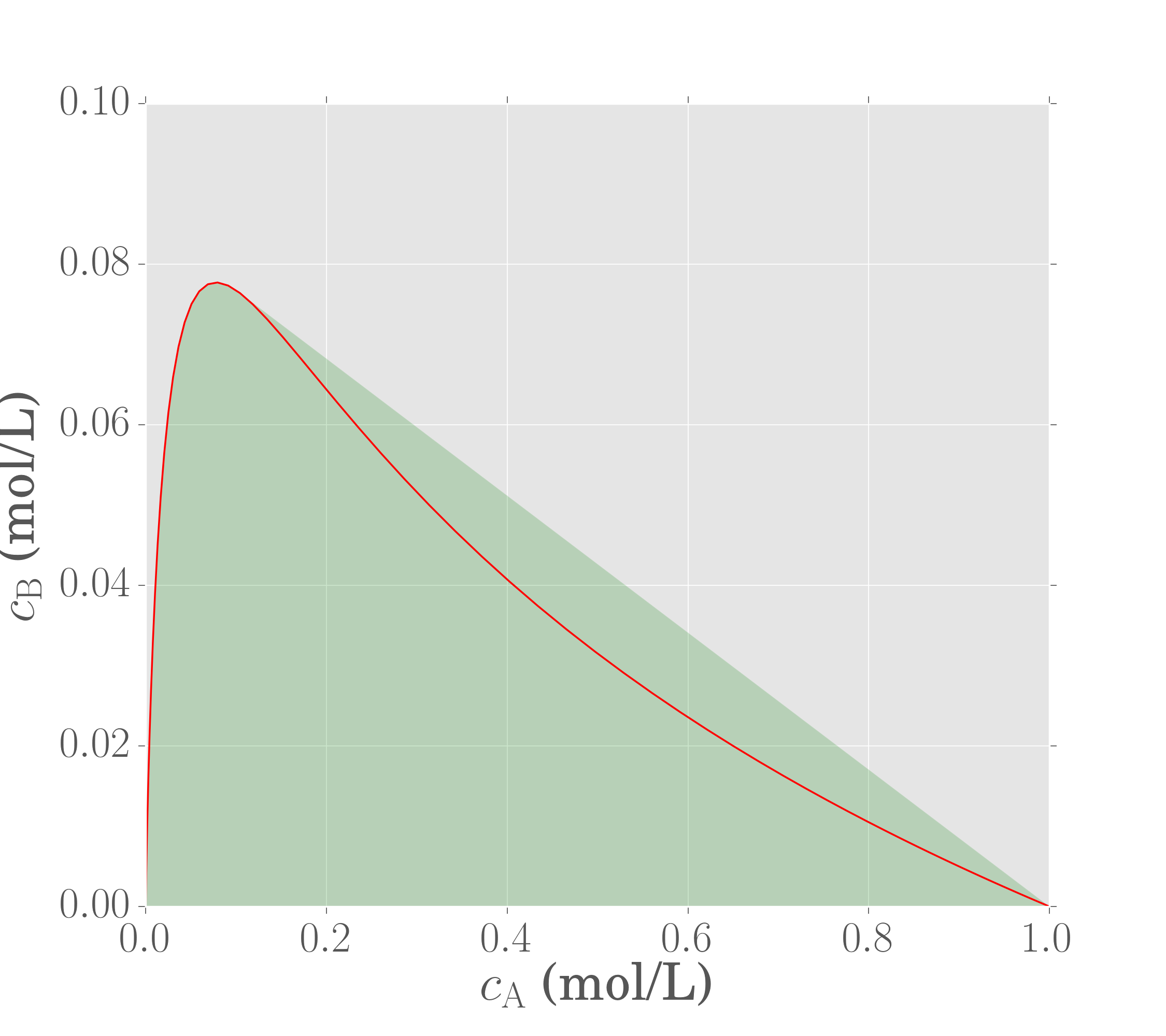
If we now compute the convex hull of the PFR points, the following convex region is generated

Jupyter notebook for PFR trajectory

Recall again that the convex hull in AR theory represents the set of achievable concentrations obtained through mixing. Thus, when the convex hull of a set of points is calculated, we are including the process of mixing into the reactor structure. All points in the shaded region are thus achievable. We've generated the region by first finding the PFR trajectory from the feed and then finding the convex hull of these points.

The region shown is an attainable region since all points in the shaded space are attainable through combinations of a PFR and mixing.

CSTR from the feed

Let us now try the same approach using a CSTR from the feed. In doing so, we are assuming that a CSTR is available to use that we can feed material equal to Cf to the reactor.

The CSTR equation is given by

$$ \mathbf{C}=\mathbf{C}_{\mathrm{f}}+\tau\mathbf{r}\left(\mathbf{C}\right) $$

When written out in terms of A and B, this gives the following system of equations

$$\begin{align} c_{\mathrm{A}} &= c_{\mathrm{Af}}+\tau r_{\mathrm{A}}\left(\mathbf{C}\right) \\ c_{\mathrm{B}} &= c_{\mathrm{Bf}}+\tau r_{\mathrm{B}}\left(\mathbf{C}\right) \end{align}$$

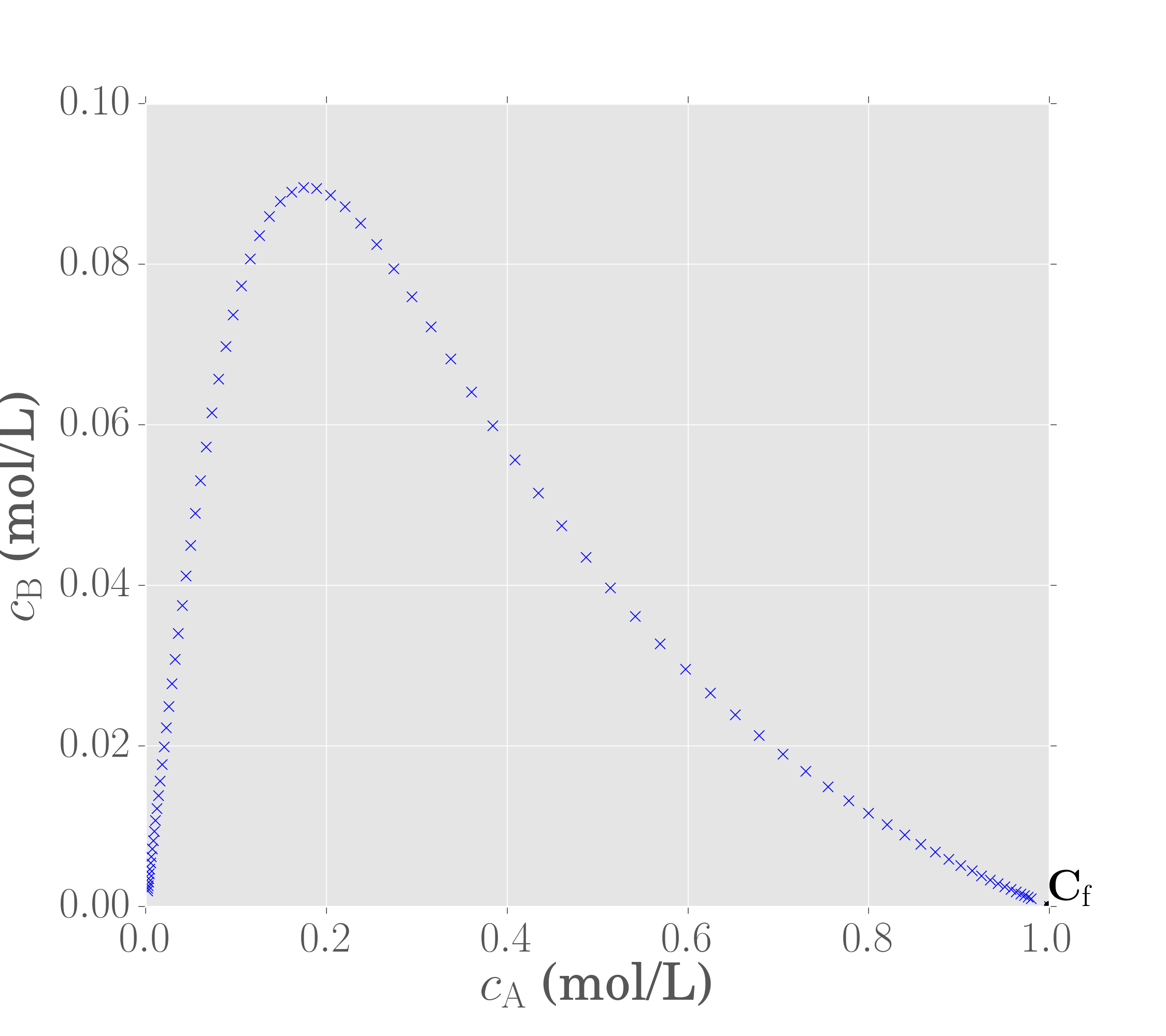
Again, we can solve this system using different residence times and plot the CSTR effluent component concentrations as a function of residence time. This is shown below.

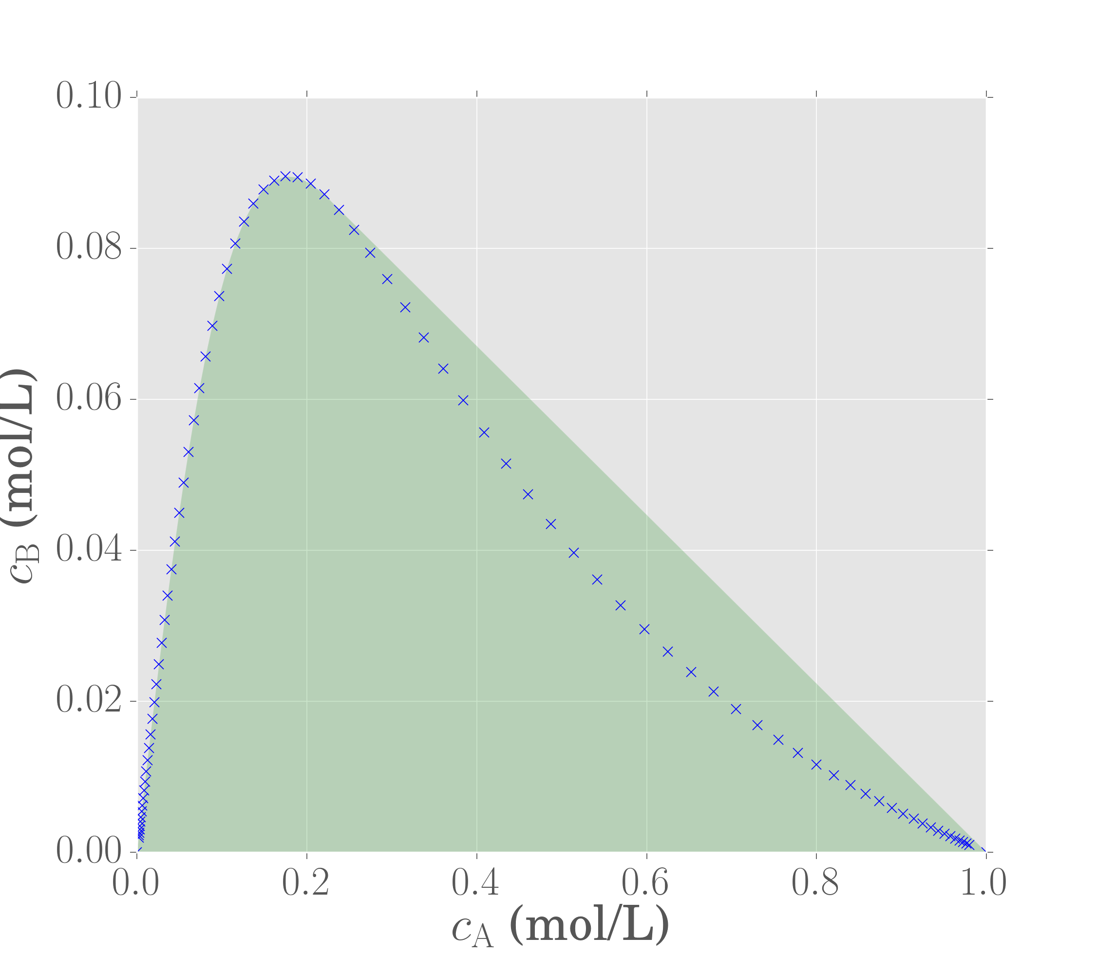
Notice that the shape of the CSTR is different to the PFR, indicating that different concentrations are achievable in a CSTR and PFR. Computing the convex hull of the CSTR points then gives the following graph:

Jupyter notebook for CSTR locus

Seeing as two reactors are available, we could plot the concentrations achievable by both reactors togther and find the convex hull of the union of both concentration sets.

This is an attainable region representing combinations of a PFR and CSTR in parallel from the feed.

Decoding reactor structures from plots (interpretting the region)

It is useful to always understand what the physical interpretation of the concentration plots are so that we know how to transform a convex region in concentration space into a physical reactor structure.

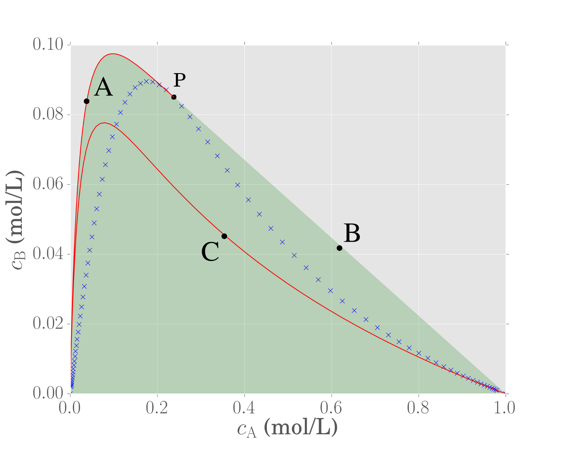
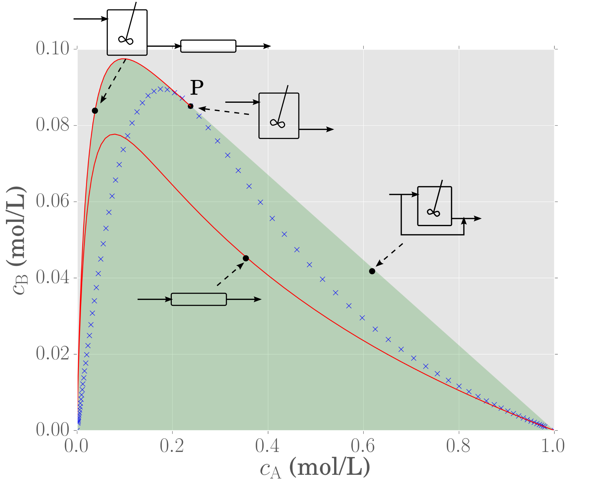
We already know the reactors associated with the red curve (PFR) and blue crosses (CSTR) since we needed to think of these reactors first before generating the region. However, these reactors are not the only possible reactor combinations that result from the region, as now we can also include mixing into the structure. Below we show three different points, labeled A, B and C. Can you figure out what type of reactor configuration is required to achieve these three points?

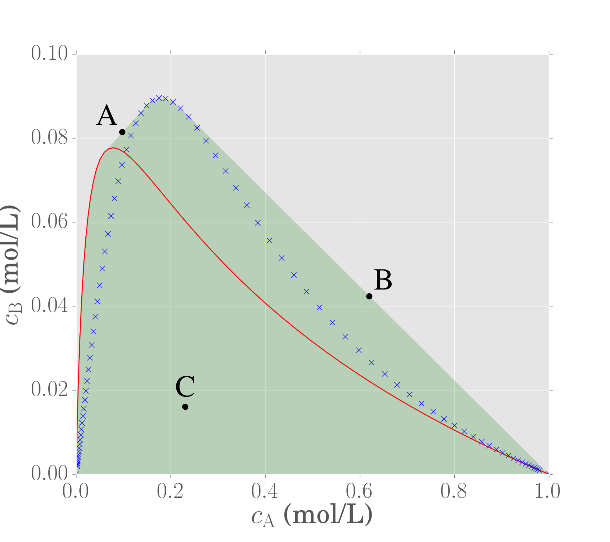
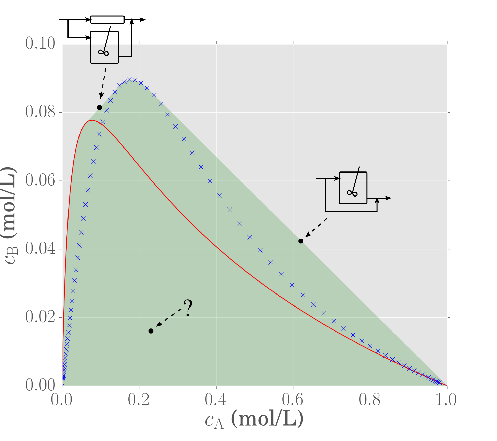
Point A is a point on the boundary that lies on a mixing line between two concentrations that originate from two physically different reactors—one of the points is from the CSTR locus from the feed point, and the other is from the PFR trajectory also initiated at the feed. Hence, point A is generated by runing a PFR and CSTR in parallel with the same feed and then mix the product streams together.

Point B is a point on the boundary that lies on a mixing line between the feed point $\mathbf{C}_\mathrm{f}$ and a point on the CSTR locus. Hence, in order to generate point B, a CSTR with bypass of fresh feed is required. Different bypass fractions will determine the specific point on this mixing line where point B will be.

Point C lies interior to the region and thus there are infinitely many ways to achieve the concentration at point C. We simply need to pick two achievable points on the boundary and draw a straight line passing through C. Thus, there is no unique reactor structure that is needed to produce point C.

Summary

Notice that the maximum concentration of B is achieved in a CSTR only. Notice also that all the reactor structures that we have discussed are the same as the scenarios given in the introduction page — a PFR from the feed, a CSTR from the feed, a CSTR with bypass, and a CSTR and PFR in parallel. The benefit of finding the AR for the system is that we can now interpret what these structures look like through geometric processes in concentration space and determine which structure performs best for a desired duty.

Although these insights are powerful, it is possible to expand the AR even further, as is demonstrated in the next section.

2b. Construct the region (part 2)

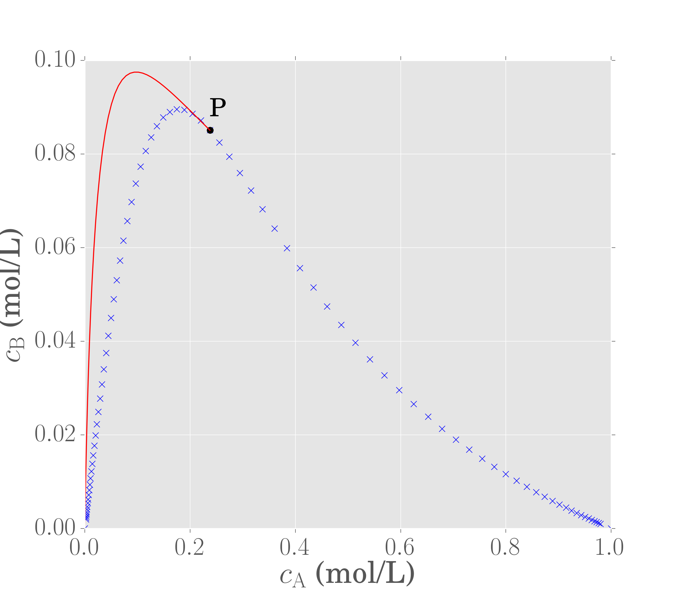
We have just generated a (convex) region representing the set of achievable concentrations for a CSTR and PFR in parallel with mixing. We can generalise this operation by observing that all points on the CSTR locus act as feed points for additional PFR trajectories, as is shown below

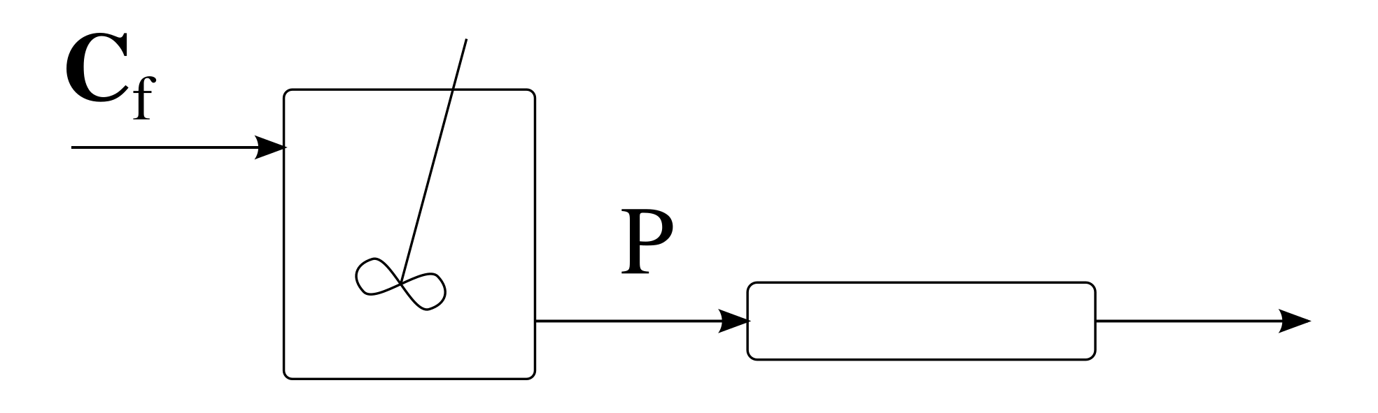
In the above illustration, a number of individual PFR trajectories are plotted from concentrations lying on the CSTR locus. Although these new trajectories (red lines) all appear to generate concentrations that extend beyond the current region, there is a specific point on the CSTR locus that generates a PFR trajectory that extends the region the greatest (it encompases all other red lines). This is marked in the figure as point P.

Since point P resides on the CSTR locus, and since the red line extending from P represents a PFR trajectory, the reactor structure required to generated these points is a CSTR from the feed with effluent concentration given by P, followed by a PFR to equilibrium.

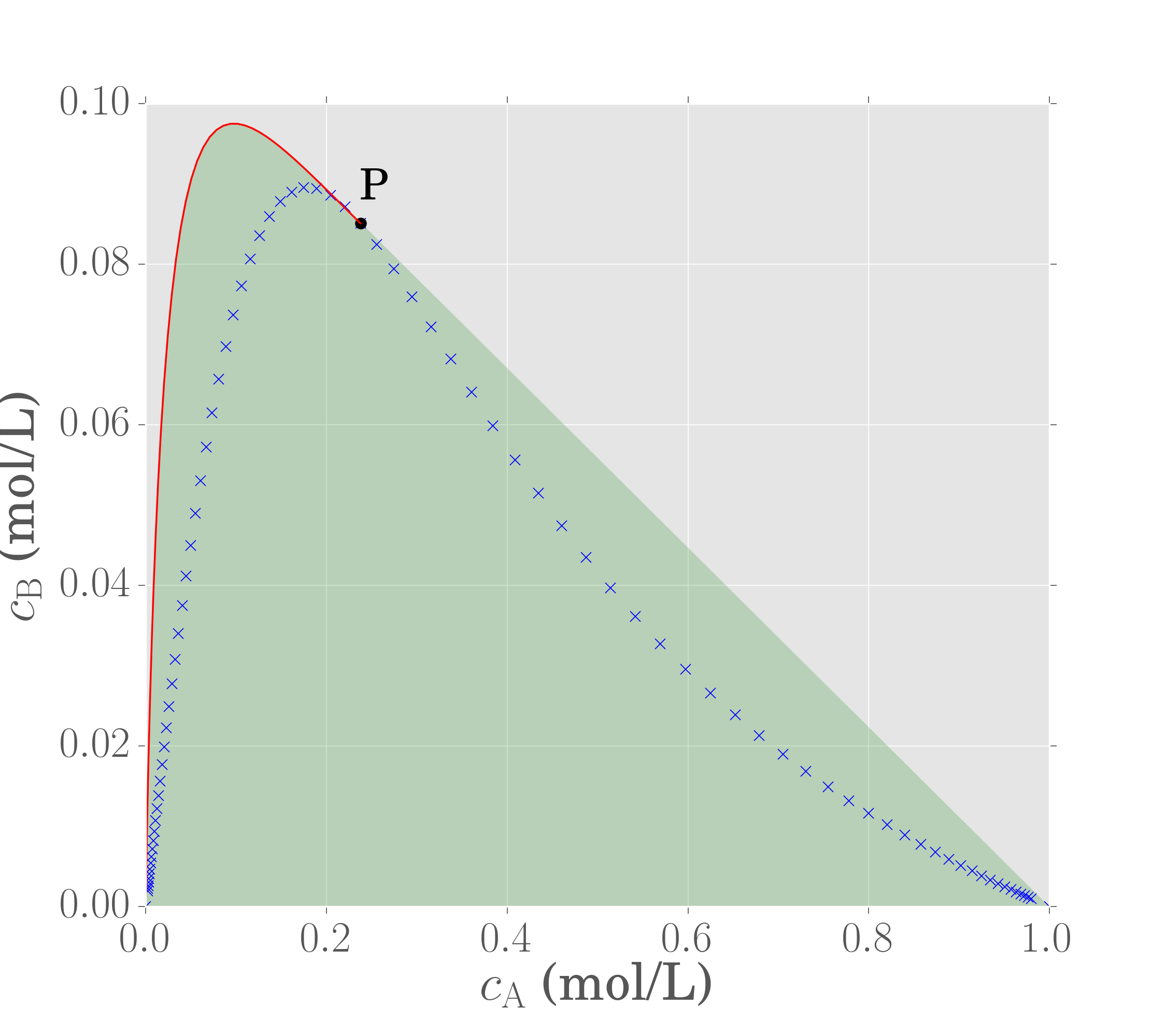
The boundary of this region is composed of only two structures:

1. A mixing line from the feed to point P
2. A PFR trajectory to point the equilibrium point (point O)

Since all rate vectors on a PFR trajectory are tangent to the trajectory, we also know that there is no possibility of extending the region further with additional PFRs.

The attainable region shown above appears to represent a large set of achievable states for the feed point and kinetics specified. How do we know that this is the complete region? For instance, what if we were to run a CSTR from somewhere inside the current region? Would this allow us to expand the region further? What if we used another PFR instead?

AR theory contains a number of important properties, which help us in determining when a region could be extended further with additional reactor types. In the next section, we will discuss a number of these properties and show that the region generated previously is in fact the true AR for this kinetics and feed point.

3. Interpret the boundary as a process flow sheet

To work out the process flowsheet required to obtain a particular product we trace the path to get to the particular point concerned. This allows us to determine the correct sequence of fundamental processes required to achieve the specified product. Again, the method is most easily understood by looking at our example.

On the diagram, remember that point P is obtained in a CSTR. For points to the right of P we require mixing of P with the system feed at O, this is then just a CSTR was bypass of feed material. Points to the left of P are obtained by following a reaction process from point P, which is achieved by adding a PFR. It can be seen that these points are obtained from a structure comprising a CSTR followed by a PFR in series.

4. Find the optimum

Once the AR has been constructed it is simple to determine the optimum for a specified objective function. The optimum is found by overlaying a contour plot of the objective function on the Attainable Region (AR) graph. That is to say we plot loci of points that have the same value of the objective function. We then identify the curve that is tangential to the AR boundary. The point where the curve of the objective function touches the boundary is the optimum operating point of the system for the specified objective function. A flowsheet to obtain this product is then the identified as discussed in the section, Interpret The Boundary As Process Structures.

Objective function 1

If we look at our example and wish to determine the maximum possible production of B, we will use the objective function:

$$ S = c_{\mathrm{B}} $$

Plotting the objective function corresponds to a horizontal line in $c_\mathrm{A}-c_\mathrm{B}$ space. The objective function is optimised when the horizontal line just touches the boundary of the AR, which, in this instance, occurs at a value of $S = 0.097$. Hence, since the objective function represents the concentration of component B, the maximum concentration of B achievable is 0.097 mol/L.

Objective function 2

We can also optimise the system for several different objective functions once the AR has been generated. For example, we may have a profit function like that given below:

$$ S=7000c_{\mathrm{B}}-500c_{\mathrm{A}}^{2} $$

In this instance, the obective function is a quadratic expression in $c_\mathrm{A}$, and thus overlaying this objective function will intersect the AR at a different point on the boundary. We find that the optimal value of $S$ in this case is when $S = 680$.

Recommended reactor structure for objective function

Once the optimal point on the AR boundary has been identified, it is simple to then to determine the process flow diagram required to achieve this optimum by interpreting the AR boundary in terms of the reactor structures that generate the boundary. The optimal design thus comes about as a consequence of finding the appropraite operating point, and not the other way around (where equipment is first selected, and then only optimised afterwards.)

Seeing as the two objective functions considered here both occur at a point beyond the critical point P, the optimal reactor structure required by both objective functions is a CSTR follwed by a PFR in series. Mixing between these reactors then generates all concentrations in the shaded region.

Take away

We have arrived at the final reactor structure by first finding what is the best performance before nominating a reactor structure. Had we started with a predefined reactor arrangement in mind first, we may have optimised and found an answer that looks appropriate, but which may not be the absolute best. The approach we adopted here was to find the answer first before finding the equipment needed to achieve this goal. Understanding how to find answers first and then only afterwards finding the corresponding reactor structures is an important factor in uncovering the truly best performance, and this is what AR theory helps us to understand.

Check the necessary conditions

So far, we have managed to generate a region in concentration space representing the set of all achievable states in a steady-state reactor network using reaction and mixing. We then proceeded to apply objective functions to the region and check for points of intersection with the boundary, as a way to optimise the system for the objective under consideration.

But how do we know that the region generated in the previous example represents all possible concentrations? That is, how do we know that there are not other reactor combinations that could expand the region further? Would a adding an extra CSTR in parallel with a PFR do anything to extend the region of achievability?

AR theory contains a number of necessary conditions that any AR must comply with. We can use these conditions as 'sanity checks' to ensure that the region generated cannot be easily extended by simple means.

In order for some region to be a candidate for the attainable region, it is required that the following necessary conditions hold.

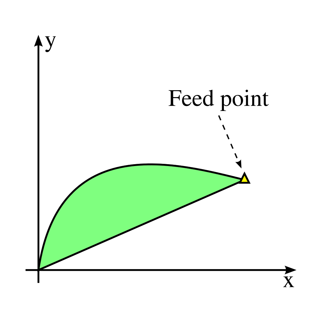
A) The region must contain all feed points

By definition, all feed points are achievable, and thus the AR must contain the feed. If there are multiple feeds present, the AR must contain all feed points.

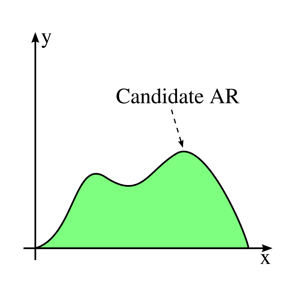
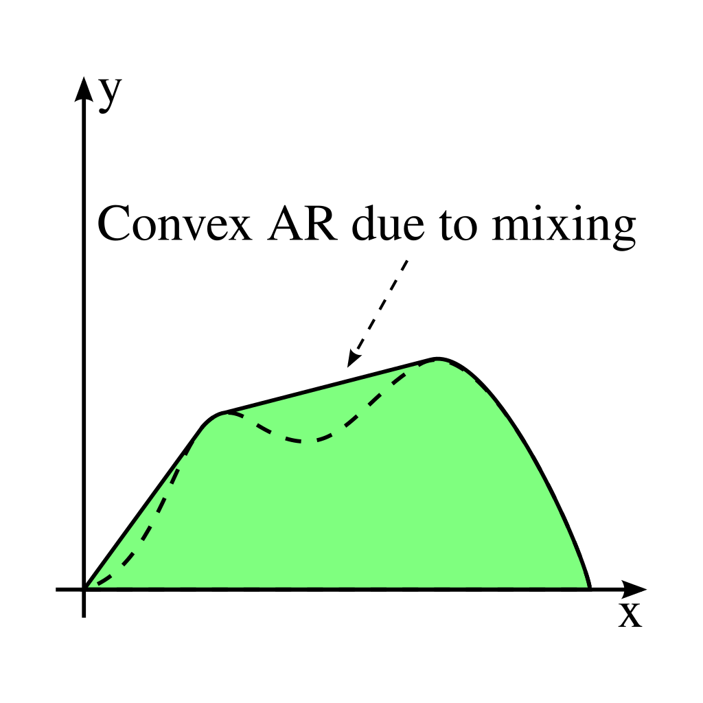
B) The AR is convex

The AR must be convex. If a region is not initially convex, it can always be made convex via the physical process of mixing. Recall that the physical interpretation of the convex hull is that of mixing, the the points belonging to the convex hull represent the unique points that may be used to generate all other points in the region via mixing.

C) No rate vectors on the AR boundary may point out of the region

Consider the following region that does not satisfy this condition for some reaction vector at a point c on the boundary of the region.

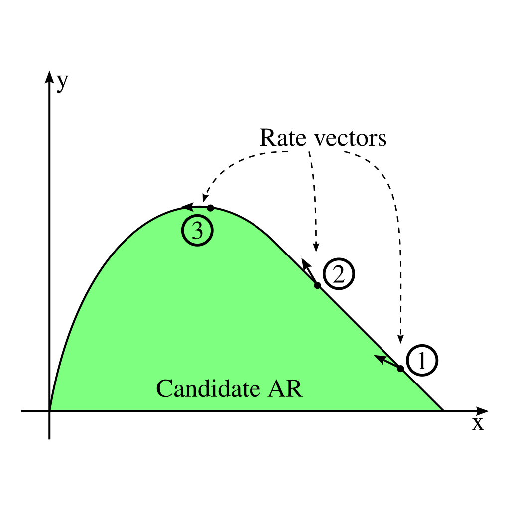
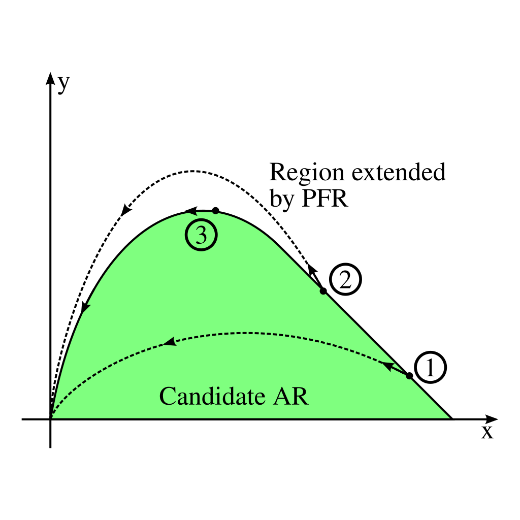
In this diagram the rate vector points outwards, thus this condition is not satisfied. We know from the section, Determining The Geometry Of The Process Units, that a PFR trajectory is tangent to the reaction vector. So, if a reaction vector points outwards at point c, we could use point c as a feed point to a PFR, and this would achieve output concentrations that lie outside of the candidate region. This allows the region to be extended and hence we have not found the region of all possible products, that is to say we have not found the complete Attainable Region.

D) No reaction vector in the complement region can be extended back so as to intersect the AR boundary

Recall that the equation for a CSTR is:

$$ \mathbf{C}=\mathbf{C}_{\mathrm{f}}+\tau\mathbf{r}\left(\mathbf{C}\right) $$

which can also be viewed as a straight line equation starting at $\mathbf{C}_\mathrm{f}$ in the (positive) direction of $\mathbf{r}\left(\mathbf{C}\right)$.

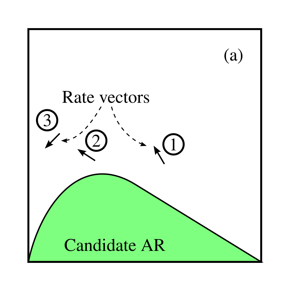
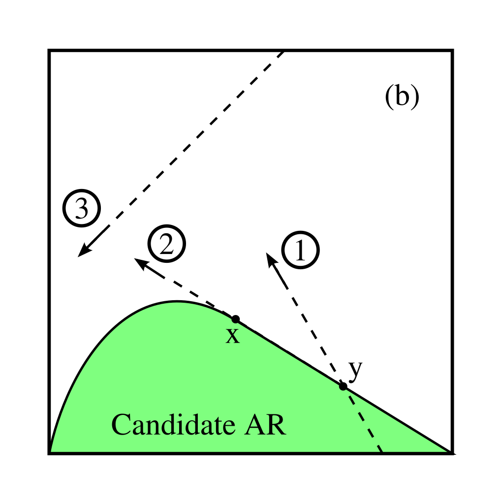
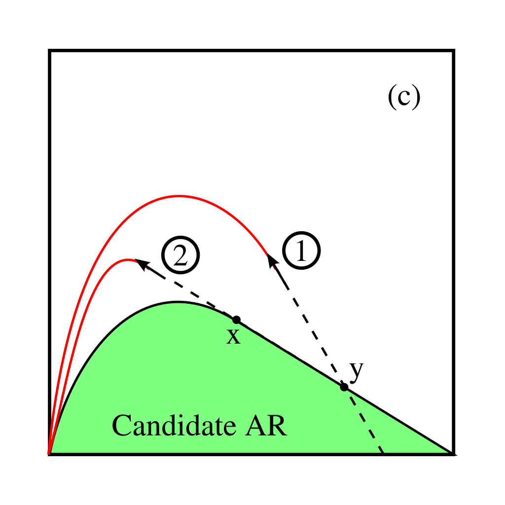
Hence, if it is possible to find a point $\mathbf{C}$ in the complement region that, when extended backwards with a straight line, intersects the region, then $\mathbf{C}$ is a CSTR solution and the region can be extended further.

Review

Check that you understand why each of these conditions must be satisfied in order for the region to be a possible attainable region.